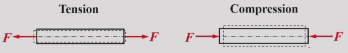
I. Concepts and Examples
The bars is subjected to a pair of longitudinal forces with equal magnitude and opposite directions, and the line of action forces coincides with the axis of the bar.
II. Internal Forces and Stress
1. Internal force
Because the action line of the external forces coincides with the axis pf the bar the action line of the internal forces also coincides with the axis of the bar, and it is called axial/normal force. The sign of axial forces is that tension is positive and compression is negative.
2. Plane cross-section hypothesis
The cross sections which were planes before deformation remain plane and perpendicular to the axis after deformation.
Under the hypothesis, we have the following conclusion:
-
The elongation of all longitudinal fibbers is equal.
-
The material is homogenous and isotropic, the internal force is evenly distributed.
-
The internal force is evenly distributed, so the normal stress at each point is constant.
So:
Then:
The normal stress has the same sign as the axial force .
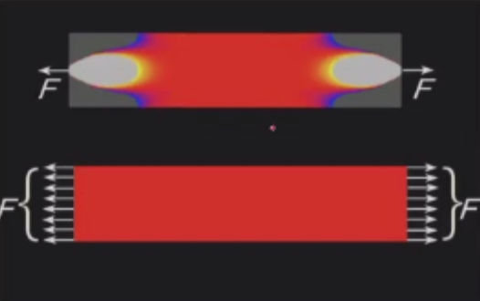
3. Saint Venant’s Principle
If a force equivalent to the distributed forces is used to replace the original force system, the effect of the above substitution is negligible at a distance from the action place of the force (about equal to the size of the cross section), except for the obvious difference in the action area of the original forces. This is Saint Venant’s principle.
III. Stresses on a Diagonal Plane
Experimental results show that the failure of a bar does not always occur along the cross section, but sometimes along diagonal planes.
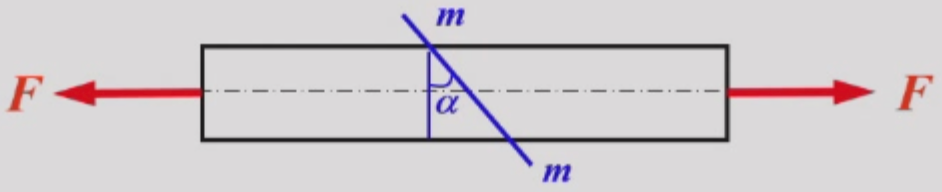
We choose the left part and study it. According to the force equilibrium and plane cross-section hypothesis, there are:
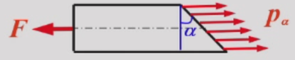 $$
F=\vec{p}_\alpha\cdot\vec{A}_\alpha=p_a A\cos \alpha
$$
Let $\sigma_0=\frac{F}{A}$, we have:
$$
p_a=\sigma_0 \cos\alpha
$$
$$
F=\vec{p}_\alpha\cdot\vec{A}_\alpha=p_a A\cos \alpha
$$
Let $\sigma_0=\frac{F}{A}$, we have:
$$
p_a=\sigma_0 \cos\alpha
$$
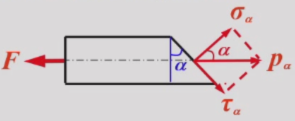
Then, we have:
They express the evolution of the normal and shear stresses on a diagonal plane in a bar that changes with angle . When , shear stress reaches the maximum value of .
IV. Mechanical Properties during Tension
1. Theory
Elastic deformation is the deformation in a test specimen from a given load disappears when the load is removed(temporary). Plastic deformation is the deformation in a test specimen from a given load remains when the load is removed(permanent).
Mechanical properties is the mechanical characteristics of materials in deformation and breaking under loads. When conducting mechanical properties testing, the following conditions must be met:
- Room temperature.
- Static load.
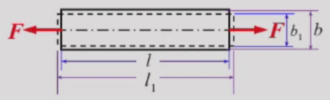
- Standard specimen: Draw two transverse lines on the bar the two ends and the distance between the lines is called gauge length , or .
After testing, we can get a series of data, the we can draw the diagram. It is related to the size of the specimen. In order to eliminate the influence of sample size, divide by the original area a of the sample to obtain the normal stress, and divide by the gauge length / to obtain the strain. According to the diagram, we can get the relation between stress and strain.
2. Example
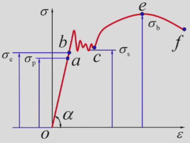
We try to study the mechanical property of a soft steel. Here are the diagram.
-
Elastic stage:
At linearly elastic stage :
is the elastic modulus. . is the proportional limit.
At non-linearly elastic stage :
is the maximum of the elastic stage.
At most time, We do not distinguish between point and . They are really close sometimes.
-
Yield stage:
When the stress exceeds point , the load is basically unchanged, but the deformation increases rapidly. This is called yield. At yield stage, the specimen loses its ability to resist deformation.
is the yield limit or yield strength.
-
Hardening stage:
After the yield stage, the specimen recovers its ability to resist deformation. To continue the deformation, the tensile force must be increased, This is called the strengthing of materials.
is the maximum of the hardening stage. is ultimate strength of ultimate limit.
-
Necking stage:
After point , the cross-sectional area of the specimen shrinks significantly in a certain place, and necking occurs until the specimen breaks.
When the specimen breaks, its elastic deformation disappears and plastic deformation remains. Its length changed from to , the original cross-dectional area is , and the minimum cross-sectional aera after fracture is . We define two plasticity indexes: Percent elongation and Percent reduction in area .
The plastic material satisfies , and brittle materials satisfies .
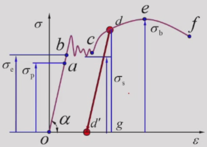
The relationship between stress and strain is linear in the unloading process, this is the law of unloading. It increases the proportional limit and decreases the percent elongation of the material, and it called cold work hardening.(The stage )
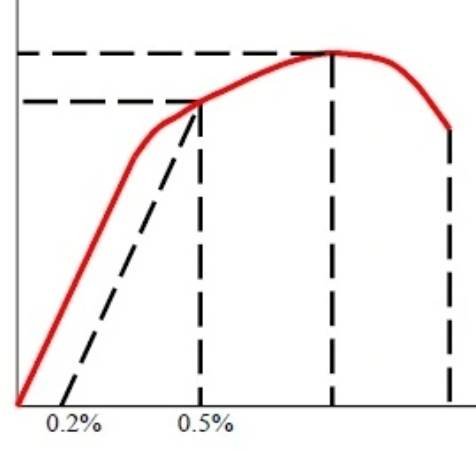
For plastic materials that don’t have an apparent yield stage, we use to define their nominal yield strength.
For the brittle materials such as cast iron, their stress-strain diagram is a slight bending curve, without yileding or necking before the sudden breaking of the specimen. The percent elongation of the are lower than .
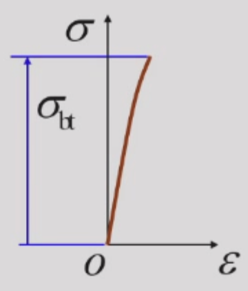
is ultimate tensile strength. It is the only strength index to evaluate the tensile strength of brittle materials.
V. Mechanical Properties during Compression
1. Theory
When we do the test, the specimen should satisfy the criteria that .
2. Example
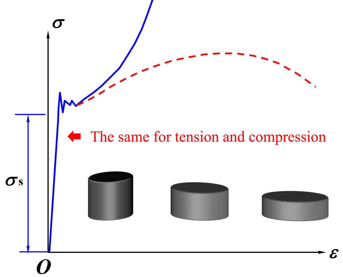
For plastic materials:
- The straight slope and yield limit of soft steel under compression are the same as under tension.
- After the yield stage, the specimen becomes flatter and the cross-sectional area keeps increasing, and is impossible for the specimen to break, so the ultimate compressive strength cannot be obtained.

For brittle materials:
-
The tensile and compressive properties of brittle materials are not identical;
-
The ultimate compressive strength is much greater than the ultimate tensile strength.
VI. Failure, Factor of Safety, Strength
1. Factor of safety and allowable stress
First, we define the working stress:
This is the actual stress generated internally within the component under real working conditions.
There are two strength indexes: (yield strength) and (ultimate strength), both are called ultimate stress, and can be expressed by , for plastic materials:
For brittle materials:
The ultimate stress is divided by a factor greater than , then the result is called allowable stress, which is expressed by :
is the factor of safety.
2. Strength conditions, strength requirements
The maximum working stress in the bar cannot exceed the allowable stress of the material:
Then we can get the allowable stress for plastic materials:
and the allowable stress for brittle materials:
According to the strength condition, three kinds of strength calculation problems can be solved:
-
For strength checking:
-
Design the cross section:
-
Determine the allowable load
VII. Deformation for Tension and Compression
1. Hooke’s law
The experomental results show that when the internal stress of in the bar does not exceed a certain limit value of the material(proportiional limit), there is:
We introduct the proportional constant :
The formula shown above is Hooke’s Law.(ceiiinosssttuv) is the tensile/compressive stiffness. The proportional constant is called elastic modulus. Elastic modulus is also called Young’s modulus. It is a physical quantity describing the ability of resist deformation of a solid material. It’s unit system is .
2. Poisson’s ratio
For longitudinal deformation and strain, we have:
For Transverse deformation and strain, we have:
We define:
as Poisson’s ratio. Experiment show that the longitudinal strain and the transverse strain is linearly proportional. For tension, longitudinal strain is positive, and the transverse strain is negative. For compression, longitudinal strain is negative, and the transverse strain is positive. Their signs are usually opposite. Classical elastic mechanics has strictly proved that the range of Poisson’s ratio of an isotropic, linearly elastic material under isothermal condition is:
VIII. Strain Energy for Tension and Compression
Strain energy is the energy stored in solid due to the deformation under the action of load. When the load decreases gradually, the deformation of the deformable body gradually recovers, and the stored strain energy is released to do work.
When :
Strain energy density is the strain energy stored in unit volume:
IX. Statically Indeterminate Problems
If the axial forces of a member cannot be obtained by static balance equations, it is called statically indeterminate problem. In other words, the number of unknown forces(internal or external) is more than the number of independent balance equations.
The key of statically indeterminate problem is compatible deformation. To solve statically indeterminate problems, in addition to equilibrium equations, it is necessary to establish geometric relationships between the displacements or deformations of various parts based on the constraints imposed by redundant supports on displacements or deformations. This involves setting up geometric equations, known as deformation compatibility equations, and establishing physical relationships between forces and displacements or deformations, i.e., physical equations or constitutive equations. Only by combining these two can the supplementary equations required for solving statically indeterminate problems be obtained.
Solving statically indeterminate problems requires a comprehensive consideration of three aspects: equilibrium, deformation compatibility, and physical relationships. This is the fundamental method for solving statically indeterminate problems.
We use to represent the number of unknown forces, which determines the indeterminate number.
TIPSteps for solving statically indeterminate problems:
- Determine the degree of static indeterminacy; write the static equilibrium equations.
- Write the deformation compatibility equations based on the deformation compatibility conditions.
- Substitute the relationship between deformation and force (Hooke’s Law) into the deformation compatibility equations to obtain the supplementary equations.
- Solve simultaneously the supplementary equations and the static equilibrium equations.
X. Thermal Stress and Assembly Stress
1. Thermal Stress
A change in temperature will cause an object to expand or shrink. Statically determinate structures can deform freely and will not cause internal forces, but in statically indeterminate structure, the deformation will be partially or completely constrained. When the temperature changes, the internal force is often caused, and the corresponding stress is called thermal stress.
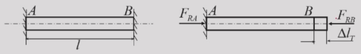
The unknown forces is:
So the thermal stress is:
2. Assembly stress
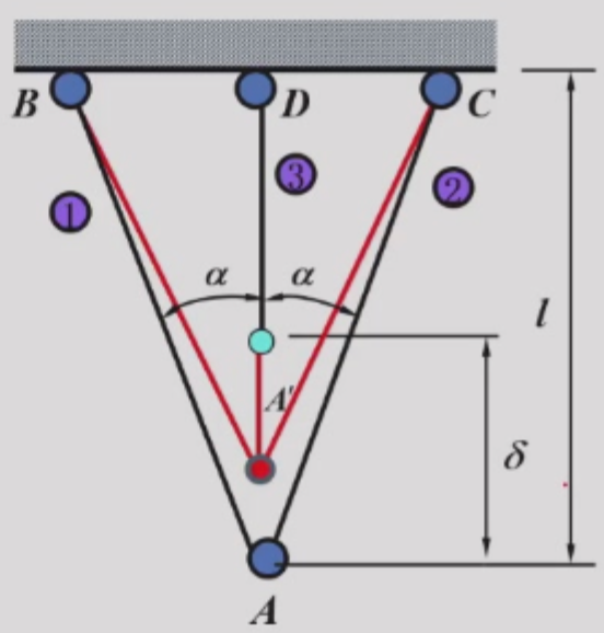
In the rod system shown, if the dimensions of the three members contain small discrepancies, then after assembly each member will occupy the positions depicted, thereby generating axial forces. The axial force in member 3 is tensile, while the axial forces in members 1 and 2 are compressive. These additional internal forces are referred to as assembly-induced internal forces, and the corresponding stresses are called assembly stresses.
We try to get the assembly stresses. First, we have the balance equation:
According to the deformation compatibility:
And we have the supplementary equation:
Then we can solve them:
XI. Stress Concentration
When a structural member contains a discontinuity, such as a hole or a sudden change in cross section, high localized stresses can occur, this is called stress concentration. We define the stress concentration factor to describe the degree of stress concentration:
The is the average stress. The sharper the size changes, or the sharper the angle is, or the smaller the hole is, the more serious the hole is, the more serious the stress concentration.
Stress concentration has much larger influence on brittle materials than the plastic materials.
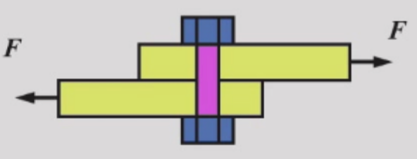
XII. Shearing and Bearing
1. Simple calculation of shearing problems

The bar is subjected to a pair of transverse forces with equal magnitude and opposite directions, and the distance between the lines of action of the forces is infinitesimal. It is called shearing.
NOTECharacteristic of deformation:
The cross section between the two forces have relative dislocation. Part of the member moves relatively along the interface of two force system.
When we meet simple calculation of shearing problems, assuming that the shear stress is uniformly distributed on the shear plane, the practical shear stress can be calculated by:
And we use to represent allowable shear stress, to represent ultimate shear stress.
2. Simple calculation of bearing problems
The local pressure occurring between bolt and steel plate is called bearing. The bearing force is:
Assuming that the normal stress is uniformly distributed on the bearing plane, the practical bearing stress can be calculated by:
And we use to represent allowable shear stress.
部分信息可能已经过时